Tutorial 1 - Creating a Model

This tutorial shows how to create a simple finite element model from scratch

The preparation stage

Before building a model, we need to load the used components. Every model needs one System instance. Furthermore, we are going to use several Node and Element instances.

Loading those class definitions requires the following:

from femedu.domain import System, Node
from femedu.elements.linear import Truss
from femedu.materials import ElasticSection

The first line imports the System and Node class definitions, the second line imports the Truss from the linear package, i.e., the small deformation finite element on variational base.

Start by creating a System instance.

model = System()

The model object will hold all information forming your finite element model, as well as provide the interface for analysis control, plotting, and data gathering.

Next, we are creating nodes as Node objects.

nd0 = Node( 0.0, 0.0)
nd1 = Node( 8.0, 6.0)
nd2 = Node(16.0, 0.0)

It is important to understand that nd0, nd1, nd2 are instances of Node and provide a permanent pointer to those nodes and all their information throughout the entire analysis. We will use those pointers to collect data or make control decisions.

We also need to add those node objects to our model.

model.addNode(nd0, nd1, nd2)

nodes can be added one at a time or, as shown above, as a group of nodes.

Every node holds information about

Type	Description	Access through
Position	initial coordinates of the node	getPos()
Displacement	current displacement components	getDisp([‘ux’, …])
Attached elements	Pointers to all connected elements	internal
Available dofs	Union of dofs used by any of the attached elements	internal
Index for a dof	Global index for locating each nodal dof in system arrays.	getIdx4DOFs(dof-list)
Index for one attached element	Global index array for locating element-specific dofs in system arrays.	getIdx4Element(elem)

Once nodes have been created, we can create and add elements to the model. This can be done by creating an element as

# define material parameters
params = dict(
    E = 1000.,   # Young's modulus
    A = 1.0,     # cross section area
)

elem0 = Truss(nd0, nd1, ElasticSection(params))

and adding that element to the model using

model.addElement(elem0)

or by creating and adding elements in one single step

model.addElement(Truss(nd1, nd2, ElasticSection(params)))

The first option allows us to keep elem0 as element pointer for later access to that element. The second option is sufficient in most cases.

FEM.edu also provides a short version for the addElement() function in the form

model += Truss(nd0, nd2, ElasticSection(params))

Note

In FEM.edu, every material instance holds information about the current state of the material, including strain, stress, plastic strain, hardening parameters, and more. Since these are private to any particular material point, each element requires its own material instance.

Creating one instance of AnyMaterial(params)() and handing that instance to the element constructor will most likely lead to a faulty model.

Geometric boundary conditions are applied at nodes. In order to add a geometric boundary condition to a node, we need to use the node pointer, i.e., the variable holding the Node instance.

In this example, we shall model nd0 as fixed and nd2 as a horizontal roller.

nd0.fixDOF(['ux','uy'])   # pin
nd2.fixDOF(['uy'])        # horizontal roller

FEM.edu always identifies degrees of freedom (dofs) using a short name string. Several dofs are predefined and used by the standard elements, though user elements and user algorithms may define additional variables as long as their respective name remains unique. Built-in standard dofs are shown in the following table.

Name	Description
ux	component of displacement in the x-direction
uy	component of displacement in the y-direction
uz	component of displacement in the z-direction
rx	component of (linearized) rotation about the x-axis
ry	component of (linearized) rotation about the y-axis
rz	component of (linearized) rotation about the z-axis

Now we are ready to load the model. This example shall be limited to simple nodal loads. For examples of more complex load patters refer to Tutorial 2 - Loading a Model

nd1.addLoad([-1.0],['uy'])

We may want to review the model status before engaging in any analysis. The easiest way is to request a report about the current state of the model as follows.

Warning

A call to model.report() may result in a lot of output if you are working on a large model.

model.report()

System Analysis Report
=======================

Nodes:
---------------------
  Node_4148:
      x:    [0. 0.]
      fix:  ['ux', 'uy']
      u:    None
  Node_4149:
      x:    [8. 6.]
      P:    [ 0. -1.]
      u:    None
  Node_4150:
      x:    [16.  0.]
      fix:  ['uy']
      u:    None

Elements:
---------------------
  Truss: Node_4148 to Node_4149:
      material properties: ElasticSection(Material)({'E': 1000.0, 'A': 1.0, 'nu': 0.0, 'fy': 1e+30, 'I': 1.0})  strain:{'axial': 0.0, 'flexure': 0.0}   stress:{'axial': 0.0, 'flexure': 0.0}
      internal force: 0.0
  Truss: Node_4149 to Node_4150:
      material properties: ElasticSection(Material)({'E': 1000.0, 'A': 1.0, 'nu': 0.0, 'fy': 1e+30, 'I': 1.0})  strain:{'axial': 0.0, 'flexure': 0.0}   stress:{'axial': 0.0, 'flexure': 0.0}
      internal force: 0.0
  Truss: Node_4148 to Node_4150:
      material properties: ElasticSection(Material)({'E': 1000.0, 'A': 1.0, 'nu': 0.0, 'fy': 1e+30, 'I': 1.0})  strain:{'axial': 0.0, 'flexure': 0.0}   stress:{'axial': 0.0, 'flexure': 0.0}
      internal force: 0.0

Things to note in this report:

• FEM.edu assigns unique names to nodes and elements. These are mostly internal identifiers but may be used by the user when analyzing/debugging program output. It is recommended to use your own node and element references to access node and element data.

• Nodes always report their reference position, but will also report fixed dofs or applied nodal loads if either was assigned to a node.

• Once an analysis has been performed, nodes will also show their current state of displacement.

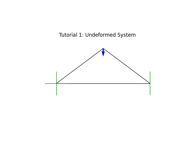
Another easy validation of your input can be obtained using the built-in system plot.

#model.resetDisp()
model.plot(factor=0.0,
           title="Tutorial 1: Undeformed System",
           show_bc=True, show_loads=True, show_reactions=False)

At this point we are ready for the analysis. Since this is a linear model, we will use the default solver, which is a LinearSolver object.

All we need to perform the analysis is

model.solve()

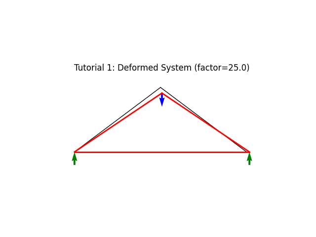
At this point, we may just plot the deformed system

model.plot(factor=25.0,
           title="Tutorial 1: Deformed System (factor=25.0)",
           filename="tutorial01_deformed.png",
           show_loads=True, show_reactions=True)

Note

Providing the filename= option will save the generated figure a file with the given name. The name may include a full path, specifying a destination folder and filename. If no path is given, the figure file will be saved to the current runtime folder.

The image file type is determined from the extension in the filename option. It is recommended to used “.pdf” for best quality (vector graphics for use in publications) or “.png” for web presentation. Avoid “.jpg” for line-graphics like this one.

model.report()

System Analysis Report
=======================

Nodes:
---------------------
  Node_4148:
      x:    [0. 0.]
      fix:  ['ux', 'uy']
      u:    [0. 0.]
  Node_4149:
      x:    [8. 6.]
      P:    [ 0. -1.]
      u:    [ 0.00533333 -0.021     ]
  Node_4150:
      x:    [16.  0.]
      fix:  ['uy']
      u:    [0.01066667 0.        ]

Elements:
---------------------
  Truss: Node_4148 to Node_4149:
      material properties: ElasticSection(Material)({'E': 1000.0, 'A': 1.0, 'nu': 0.0, 'fy': 1e+30, 'I': 1.0})  strain:{'axial': -0.0008333333333333333}   stress:{'axial': -0.8333333333333333, 'flexure': 0.0}
      internal force: -0.8333333333333333
  Truss: Node_4149 to Node_4150:
      material properties: ElasticSection(Material)({'E': 1000.0, 'A': 1.0, 'nu': 0.0, 'fy': 1e+30, 'I': 1.0})  strain:{'axial': -0.0008333333333333333}   stress:{'axial': -0.8333333333333333, 'flexure': 0.0}
      internal force: -0.8333333333333333
  Truss: Node_4148 to Node_4150:
      material properties: ElasticSection(Material)({'E': 1000.0, 'A': 1.0, 'nu': 0.0, 'fy': 1e+30, 'I': 1.0})  strain:{'axial': 0.0006666666666666664}   stress:{'axial': 0.6666666666666664, 'flexure': 0.0}
      internal force: 0.6666666666666664

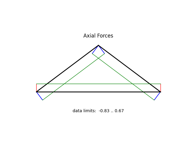
Truss, beam, and frame elements further allow for plotting of internal forces through the beamValuePlot(variable,factor=1.0,filename=’…’) method.

Valid variables are

‘F’	Axial force (tension positive)
‘V’	transverse shear force
‘M’	Bending moment

model.beamValuePlot('F',filename='tutorial01_axial.png')