Example: plate02

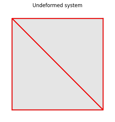
Initial system and meshing for the patch test.

We build the model based a few parameters as follows.

        params = dict(
            E  = 10.,   # Young's modulus
            nu = 0.3,   # Poisson's ratio
            t  = 1.0,   # thickness of the plate
            fy = 1.e30  # yield stress
        )

        a = 10.     # length of the plate in the x-direction
        b = 10.     # length of the plate in the y-direction

All mesh creation is based solely on the above parameters to allow for easy manipulation of the model.

The actual model is built by the block below.

        model = System()
        model.setSolver(NewtonRaphsonSolver())

        nd0 = Node( 0.0, 0.0)
        nd1 = Node(   a, 0.0)
        nd2 = Node(   a,   b)
        nd3 = Node( 0.0,   b)

        nd0.fixDOF('ux', 'uy')
        nd1.fixDOF('uy')
        nd3.fixDOF('ux')

        model.addNode(nd0, nd1, nd2, nd3)

        elemA = LinearTriangle(nd0, nd1, nd3, PlaneStress(params))
        elemB = LinearTriangle(nd2, nd3, nd1, PlaneStress(params))

        model.addElement(elemA, elemB)

        elemB.setSurfaceLoad(face=2, w=1.0)

Line 10 instantiates one model space.

Line 11 switches from the default linear solver to the NewtonRaphsonSolver, needed for nonlinear problems.

Lines 13-16 create the nodes, and lines 18 adds them to the model space.

Lines 18-20 apply the geometric boundary condition. This examples implements symmetry conditions at \(x=0\) and \(y=0\).

Lines 24-25 create the elements and line 27 adds them to the model space. You only need to create variables for Node and Element objects, respectively, if you need to either add or retrieve information from that object later.

Lines 29 adds a surface load to face 2 of element elemB. See Triangle class for the definition of faces for this element.

We initialize the system by solving for load-level 0.00. This is not necessary for most models, though some thermo-elastic or elast-plastic problems, e.g., may not be in equilibrium in an undeformed state. The cost is minimal and adding this step to a nonlinear analysis is a good habit. The system equations are solved by a single call to the solver:

        model.setLoadFactor(0.0)
        model.solve()
        #model.report()  # activate this line for lots of debug info
        model.plot(factor=1.0,
                   title="Undeformed system",
                   filename="plate02_undeformed.png")

Next increase the load to the next target load-level, here we are using 1.0 (100% of the reference load). The system equations are once again solved by a single call to the solver:

        model.setLoadFactor(1.0)
        model.solve()
        model.plot(factor=1.0, filename="plate02_deformed.png")

The solver report the residual norm during each step. The geometric nonlinearity of the element requires multiple iteration steps before achieving equilibrium. The following convergence print-out shows that the element generates a quadratic rate of convergence when paired with the NewtonRaphsonSolver.

norm of the out-of-balance force:   7.0711e+00
norm of the out-of-balance force:   1.1554e+00
norm of the out-of-balance force:   1.7307e-02
norm of the out-of-balance force:   4.2408e-06
norm of the out-of-balance force:   2.2995e-13

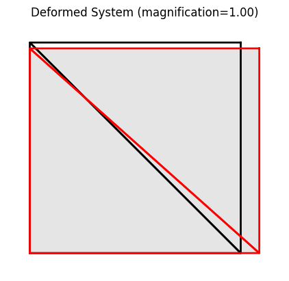
Deformed system at load level 1.00

You can obtain a debug-style report on the state of the system:

        model.report()

The report looks like this:

System Analysis Report
=======================

Nodes:
---------------------
  Node_0:
      x:    [0. 0.]
      fix:  ['ux', 'uy']
      u:    [0. 0.]
  Node_1:
      x:    [10.  0.]
      fix:  ['uy']
      u:    [0.88033915 0.        ]
  Node_2:
      x:    [10. 10.]
      u:    [ 0.88033915 -0.27963653]
  Node_3:
      x:    [ 0. 10.]
      fix:  ['ux']
      u:    [ 0.         -0.27963653]

Elements:
---------------------
  LinearTriangle: nodes ( Node_0 Node_1 Node_3 )
      material: PlaneStress
      strain: xx=9.191e-02 yy=-2.757e-02 xy=0.000e+00 zz=-1.930e-02
      stress: xx=9.191e-01 yy=2.054e-15 xy=0.000e+00 zz=0.000e+00
  LinearTriangle: nodes ( Node_2 Node_3 Node_1 )
      material: PlaneStress
      strain: xx=9.191e-02 yy=-2.757e-02 xy=1.727e-16 zz=-1.930e-02
      stress: xx=9.191e-01 yy=3.886e-15 xy=6.641e-16 zz=0.000e+00
      element forces added to node:
          Node_2: [5. 0.]
          Node_3: [0. 0.]
          Node_1: [5. 0.]

Importing the example

from femedu.examples.plates.plate02 import *

# load the example
ex = ExamplePlate02()

More frame examples: Plate Examples