Example: truss01

We build the model based a few parameters as follows.

        """
        return s

    def problem(self):

All mesh creation is based solely on the above parameters to allow for easy manipulation of the model.

The actual model is built by the block below.

        B = 6.0 * 12
        H = 3.0 * 12
        params = {'E': 10., 'A': 1., 'nu': 0.0, 'fy': 1.e30}

        model = System()

        # create nodes
        nd0 = Node(0.0, 0.0)
        nd1 = Node(  B, 0.0)
        nd2 = Node(0.5*B, H)

        model.addNode(nd0, nd1, nd2)

        # create elements
        model.addElement(Truss(nd0, nd1, FiberMaterial(params)))  # bottom 1
        model.addElement(Truss(nd0, nd2, FiberMaterial(params)))  # up right diag 1
        model.addElement(Truss(nd1, nd2, FiberMaterial(params)))  # up left diag 1

        # define support(s)
        nd0.fixDOF('ux', 'uy')    # pin support left end
        nd1.fixDOF('uy')            # roller support right end

Line 5 instantiates one model space.

Lines 8-10 create the nodes, and lines 12 adds them to the model space.

Lines 14-17 create the elements and simultaneously adds them to the model space. You only need to create variables for Node and Element objects, respectively, if you need to either add or retrieve information from that object later.

Lines 19-21 define the support conditions by providing the respective information directly to the supported nodes.

Lines 23-25 applies the reference load(s) as a nodal force at nd2.

The system equations are solved by a single call to the solver:

        # add loads
        # .. load only the upper nodes

You can obtain a debug-style report on the state of the system:

        # analyze the model

Resulting in an output like (may change as the code evolves).

System Analysis Report
=======================

Nodes:
---------------------
  Node 0: {'ux': 0, 'uy': 1}
          x:[0. 0.], fix:['ux', 'uy'],
          P:[0. 0.], u:[0. 0.]
  Node 1: {'ux': 0, 'uy': 1}
          x:[72.  0.], fix:['uy', 'ux'],
          P:[0. 0.], u:[0. 0.]
  Node 2: {'ux': 0, 'uy': 1}
          x:[36. 36.], fix:[],
          P:[ 0. -1.], u:[ 0.         -5.09116882]

Elements:
---------------------
  Truss: node 0 to node 1:
     material properties: FiberMaterial(Material)({'E': 10.0, 'A': 1.0, 'nu': 0.0, 'fy': 1e+30})  strain:0.0   stress:{'xx': 0.0, 'yy': 0.0, 'zz': 0.0, 'xy': 0.0}
     internal force: 0.0
     Pe: [ 0.0 0.0 ]
  Truss: node 0 to node 2:
     material properties: FiberMaterial(Material)({'E': 10.0, 'A': 1.0, 'nu': 0.0, 'fy': 1e+30})  strain:-0.06989658167930027   stress:{'xx': -0.6989658167930026, 'yy': 0.0, 'zz': 0.0, 'xy': 0.0}
     internal force: -0.6989658167930026
     Pe: [ -0.530317996923979 -0.4553197065619366 ]
  Truss: node 1 to node 2:
     material properties: FiberMaterial(Material)({'E': 10.0, 'A': 1.0, 'nu': 0.0, 'fy': 1e+30})  strain:-0.06989658167930027   stress:{'xx': -0.6989658167930026, 'yy': 0.0, 'zz': 0.0, 'xy': 0.0}
     internal force: -0.6989658167930026
     Pe: [ 0.530317996923979 -0.4553197065619366 ]

An easier way to look at the simulation results are plots. A deformed system plot is obtained using the model.plot() directive. If a filename is given, the plot will be saved to the harddrive using that file name. An internal force plot is created equally simple.

        # write out report
        model.report()

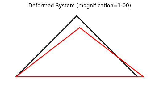
Showing file truss01_deformed.png

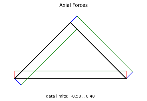
Showing file truss01_forces.png

Importing the example

from femedu.examples.trusses.truss01 import *

# load the example
ex = ExampleTruss01()

More truss examples: Truss Examples