Example: truss03

We build the model based a few parameters as follows.

        # initialize a system model
        B = 6.0 * 12
        H = 3.0 * 12
        params = {'E': 10., 'A': 1., 'nu': 0.0, 'fy': 1.e30}

All mesh creation is based solely on the above parameters to allow for easy manipulation of the model.

The actual model is built by the block below.

        model = System()

        # create nodes
        nd0 = Node(0.0, 0.0)
        nd1 = Node(  B, 0.0)
        nd2 = Node(0.5*B, H)

        model += nd0
        model += nd1
        model += nd2

        # create elements
        model += Truss(nd0, nd1, FiberMaterial(params))  # bottom 1
        model += Truss(nd0, nd2, FiberMaterial(params))  # up right diag 1
        model += Truss(nd1, nd2, FiberMaterial(params))  # up left diag 1

        # define support(s)
        nd0.fixDOF('ux')    # horizontal support left end
        #nd0 //= 0
        nd0.fixDOF('uy')    # vertical support left end
        nd1.fixDOF('uy')    # vertical support right end

        # add loads
        # .. load only the upper nodes
        nd2.setLoad((0.0, -1.0), ('ux','uy'))

Line 5 instantiates one model space.

Lines 8-10 create the nodes, and lines 12-14 add them to the model space.

Lines 16-19 create the elements and simultaneously adds them to the model space. You only need to create variables for Node and Element objects, respectively, if you need to either add or retrieve information from that object later.

Lines 21-25 define the support conditions by providing the respective information directly to the supported nodes.

Lines 27-29 applies the reference load(s) as a nodal force at nd2.

The system equations are solved by a single call to the solver:

        # analyze the model
        model.solve()

You can obtain a debug-style report on the state of the system:

        # write out report
        model.report()

Resulting in an output like (may change as the code evolves).

System Analysis Report
=======================

Nodes:
---------------------
  Node 0: {'ux': 0, 'uy': 1}
          x:[0. 0.], fix:['ux', 'uy'],
          P:[0. 0.], u:[0. 0.]
  Node 1: {'ux': 0, 'uy': 1}
          x:[72.  0.], fix:['uy', 'ux'],
          P:[0. 0.], u:[0. 0.]
  Node 2: {'ux': 0, 'uy': 1}
          x:[36. 36.], fix:[],
          P:[ 0. -1.], u:[ 0.         -5.09116882]

Elements:
---------------------
  Truss: node 0 to node 1:
     material properties: FiberMaterial(Material)({'E': 10.0, 'A': 1.0, 'nu': 0.0, 'fy': 1e+30})  strain:0.0   stress:{'xx': 0.0, 'yy': 0.0, 'zz': 0.0, 'xy': 0.0}
     internal force: 0.0
     Pe: [ 0.0 0.0 ]
  Truss: node 0 to node 2:
     material properties: FiberMaterial(Material)({'E': 10.0, 'A': 1.0, 'nu': 0.0, 'fy': 1e+30})  strain:-0.06989658167930027   stress:{'xx': -0.6989658167930026, 'yy': 0.0, 'zz': 0.0, 'xy': 0.0}
     internal force: -0.6989658167930026
     Pe: [ -0.530317996923979 -0.4553197065619366 ]
  Truss: node 1 to node 2:
     material properties: FiberMaterial(Material)({'E': 10.0, 'A': 1.0, 'nu': 0.0, 'fy': 1e+30})  strain:-0.06989658167930027   stress:{'xx': -0.6989658167930026, 'yy': 0.0, 'zz': 0.0, 'xy': 0.0}
     internal force: -0.6989658167930026
     Pe: [ 0.530317996923979 -0.4553197065619366 ]

An easier way to look at the simulation results are plots. A deformed system plot is obtained using the model.plot() directive. If a filename is given, the plot will be saved to the harddrive using that file name.

        # create plots
        model.plot(factor=1., filename="truss03_deformed_a.png")

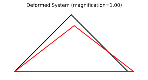
Showing file truss03_deformed_a.png

Analyzing a variation of this system

Studying a variation of a system is rather easy once a model has been generated. Let us modify the system by fixing the horizontal movement of node 1 in addition to the existing constraints (Line 37).

We also have to reset the displacements (Line 42) to reinitialize the analysis.

        # fix horizontal motion of node 1
        nd1.fixDOF('ux')

        # add loads: same load -- nothing to do

        # RE-analyze the model
        model.resetDisp()
        model.solve()

        # skip the report
        model.report()

        # create plots
        model.plot(factor=1., filename="truss03_deformed_b.png")

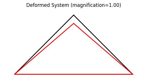
Showing file truss03_deformed_b.png. Note that neither of the bottom nodes moves after modifying the support.

Importing the example

You can import and run this example from the distribution as follows.

from femedu.examples.trusses.truss03 import *

# load the example
ex = ExampleTruss03()

More truss examples: Truss Examples