Example: truss02
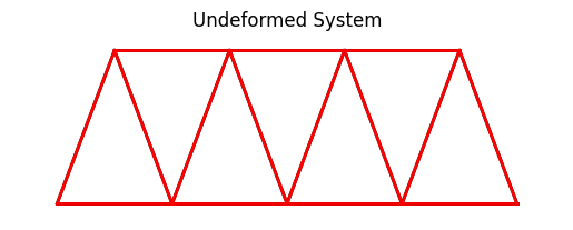
System and deformed shape
We build the model based a few parameters as follows.
1        # initialize a system model
2        P = -10.0      # reference load on top nodes
3        B = 6.0 * 12   # with of one bay in inches
4        H = 8.0 * 12   # height of one bay in inches
5
6        # material model parameters
7        params = {'E': 10000., 'A': 3., 'nu': 0.0, 'fy': 1.e30}
All mesh creation is based solely on the above parameters to allow for easy manipulation of the model.
The actual model is built by the block below.
 8        model = System()
 9        model.setSolver(NewtonRaphsonSolver())
10
11        # create nodes
12        nd0 = Node(0.0, 0.0)
13        nd1 = Node(  B, 0.0)
14        nd2 = Node(2*B, 0.0)
15        nd3 = Node(3*B, 0.0)
16        nd4 = Node(4*B, 0.0)
17        nd5 = Node(0.5*B, H)
18        nd6 = Node(1.5*B, H)
19        nd7 = Node(2.5*B, H)
20        nd8 = Node(3.5*B, H)
21
22        model.addNode(nd0, nd1, nd2, nd3, nd4, nd5, nd6, nd7, nd8)
23
24        # create elements
25        model.addElement(Truss(nd0, nd1, FiberMaterial(params)))  # bottom 1
26        model.addElement(Truss(nd1, nd2, FiberMaterial(params)))  # bottom 2
27        model.addElement(Truss(nd2, nd3, FiberMaterial(params)))  # bottom 3
28        model.addElement(Truss(nd3, nd4, FiberMaterial(params)))  # bottom 4
29
30        model.addElement(Truss(nd5, nd6, FiberMaterial(params)))  # upper 1
31        model.addElement(Truss(nd6, nd7, FiberMaterial(params)))  # upper 2
32        model.addElement(Truss(nd7, nd8, FiberMaterial(params)))  # upper 3
33
34        model.addElement(Truss(nd0, nd5, FiberMaterial(params)))  # up right diag 1
35        model.addElement(Truss(nd1, nd6, FiberMaterial(params)))  # up right diag 2
36        model.addElement(Truss(nd2, nd7, FiberMaterial(params)))  # up right diag 3
37        model.addElement(Truss(nd3, nd8, FiberMaterial(params)))  # up right diag 4
38
39        model.addElement(Truss(nd1, nd5, FiberMaterial(params)))  # up left diag 1
40        model.addElement(Truss(nd2, nd6, FiberMaterial(params)))  # up left diag 2
41        model.addElement(Truss(nd3, nd7, FiberMaterial(params)))  # up left diag 3
42        model.addElement(Truss(nd4, nd8, FiberMaterial(params)))  # up left diag 4
43
44        # define support(s)
45        nd0.fixDOF('ux', 'uy')    # horizontal support left end
46        nd4.fixDOF('uy')            # vertical support right end
47
48        # add loads
49        # .. load only the upper nodes
50        nd5.setLoad((P,), ('uy',))
51        nd6.setLoad((P,), ('uy',))
52        nd7.setLoad((P,), ('uy',))
53        nd8.setLoad((P,), ('uy',))
Line 8 instantiates one model space.
Line 9 switches from the default linear solver to the NewtonRaphsonSolver, needed for nonlinear problems.
Lines 11-20 create the nodes, and line 22 adds them to the model space.
Lines 24-42 create the elements and simultaneously adds them to the model space. You only need to create variables for Node and Element objects, respectively, if you need to either add or retrieve information from that object later.
Lines 44-46 define the support conditions by providing the respective information directly to the supported nodes.
Lines 48-53 applies the reference load(s) as a nodal force at nd2.
The system equations are solved by a single call to the solver:
54        # analyze the model
55        model.solve()
You can obtain a debug-style report on the state of the system:
56        # write out report
57        model.report()
Resulting in an output like (may change as the code evolves).
System Analysis Report
=======================

Nodes:
---------------------
  Node_0:
      x:    [0. 0.]
      fix:  ['ux', 'uy']
      u:    [0. 0.]
  Node_1:
      x:    [72.  0.]
      u:    [ 0.0175857  -0.18448191]
  Node_2:
      x:    [144.   0.]
      u:    [ 0.05359577 -0.25049274]

[ ... ]

Elements:
---------------------
  Truss: node 0 to node 1:
     material properties: FiberMaterial(Material)({'E': 10000.0, 'A': 3.0, 'nu': 0.0, 'fy': 1e+30})  strain:0.00025074648384184977   stress:{'xx': 2.5074648384184974, 'yy': 0.0, 'zz': 0.0, 'xy': 0.0}
     internal force: 7.522394515255492
     Pe: [ 7.522369834729211 -0.01926947591183249 ]
  Truss: node 1 to node 2:
     material properties: FiberMaterial(Material)({'E': 10000.0, 'A': 3.0, 'nu': 0.0, 'fy': 1e+30})  strain:0.0005007291419303546   stress:{'xx': 5.007291419303546, 'yy': 0.0, 'zz': 0.0, 'xy': 0.0}
     internal force: 15.021874257910639
     Pe: [ 15.021867950880157 -0.013765420367433319 ]
  Truss: node 2 to node 3:
     material properties: FiberMaterial(Material)({'E': 10000.0, 'A': 3.0, 'nu': 0.0, 'fy': 1e+30})  strain:0.0005007291419303549   stress:{'xx': 5.00729141930355, 'yy': 0.0, 'zz': 0.0, 'xy': 0.0}
     internal force: 15.02187425791065
     Pe: [ 15.021867950880168 0.01376542036743333 ]

[ ... ]
An easier way to look at the simulation results are plots. A deformed system plot is obtained using the model.plot() directive. If a filename is given, the plot will be saved to the harddrive using that file name. An internal force plot is created equally simple.
58        # create plots
59        model.plot(factor=20.,  filename="truss02_deformed.png")
60        model.beamValuePlot('f',filename="truss02_forces.png")
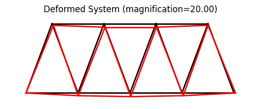
System and deformed shape
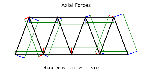
Axial force diagram
Importing the example
from femedu.examples.trusses.truss02 import *

# load the example
ex = ExampleTruss02()
More truss examples: Truss Examples