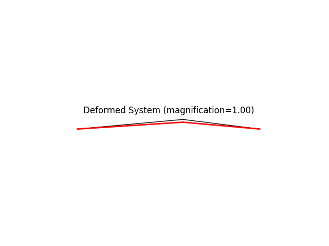
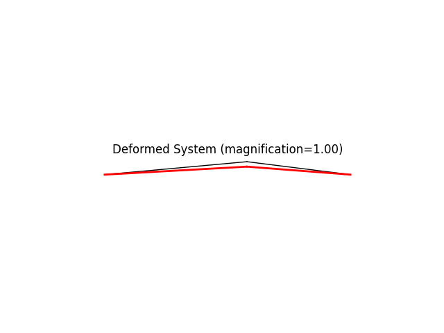
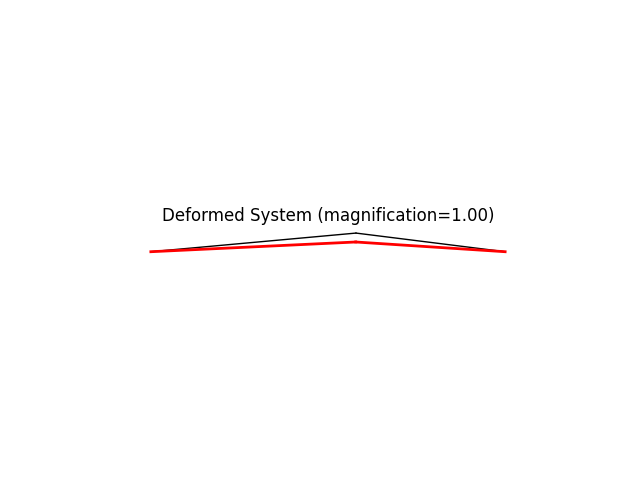
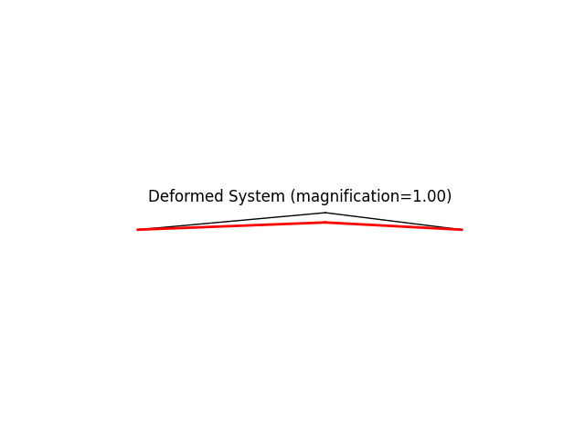
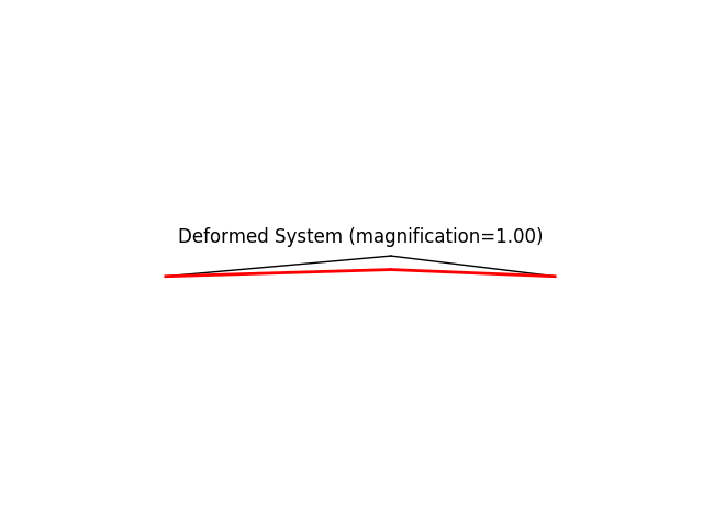
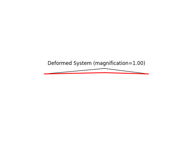
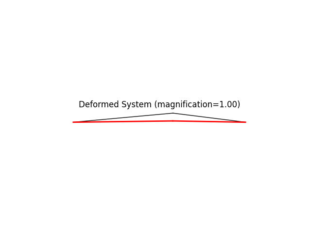
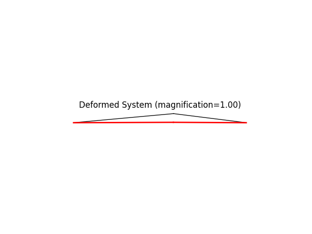
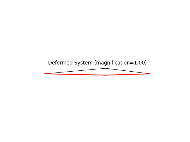
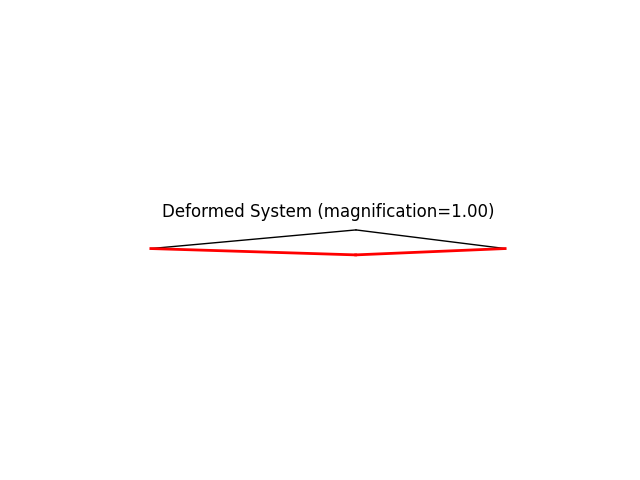
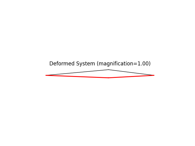
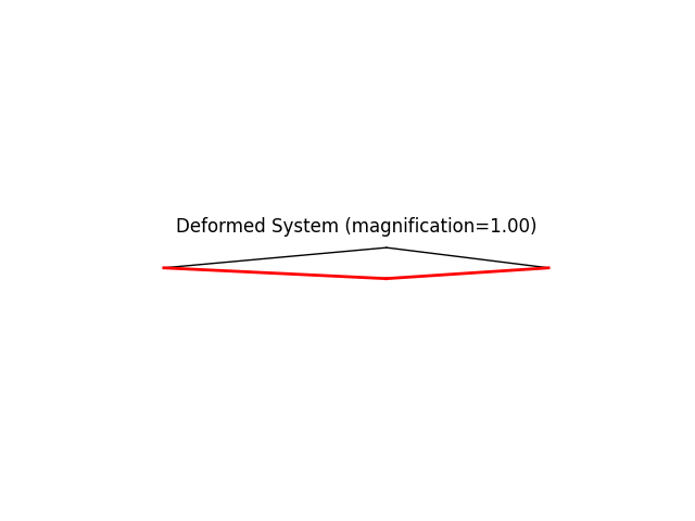
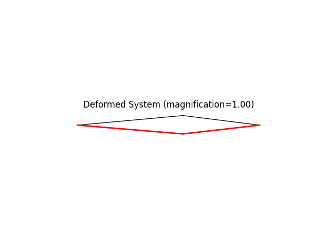
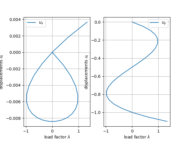
Simple triangular truss.

Study of snap-through behavior using finite deformation truss elements.

We shall be using displacement control to trace the unstable portion of the static equilibrium path.

Author: Peter Mackenzie-Helnwein

Setup

import numpy as np
import matplotlib.pyplot as plt

from femedu.examples import Example

from femedu.domain import System, Node
from femedu.elements.finite import Truss
from femedu.materials import FiberMaterial
from femedu.solver import NewtonRaphsonSolver

Create the example by subclassing the Example

class ExampleTruss06(Example):

    def problem(self):
        # initialize a system model
        model = System()
        model.setSolver(NewtonRaphsonSolver())

        # create notes
        x1=Node(0.0,0.0)
        x2=Node(5.5,0.5)
        x3=Node(9.5,0.0)

        model.addNode(x1,x2,x3)

        params = dict(
            E = 2100.,   # MOE
            A = 1.       # cross section area
        )

        # create elements
        elemA = Truss(x1,x2, FiberMaterial(params))
        elemB = Truss(x3,x2, FiberMaterial(params))

        model += elemA
        model += elemB

        # apply boundary conditions
        x1.fixDOF(['ux','uy'])
        x3.fixDOF(['ux','uy'])

        # build reference load
        x2.addLoad([-1.],['uy'])

        # write out report
        model.report()

        # create plots
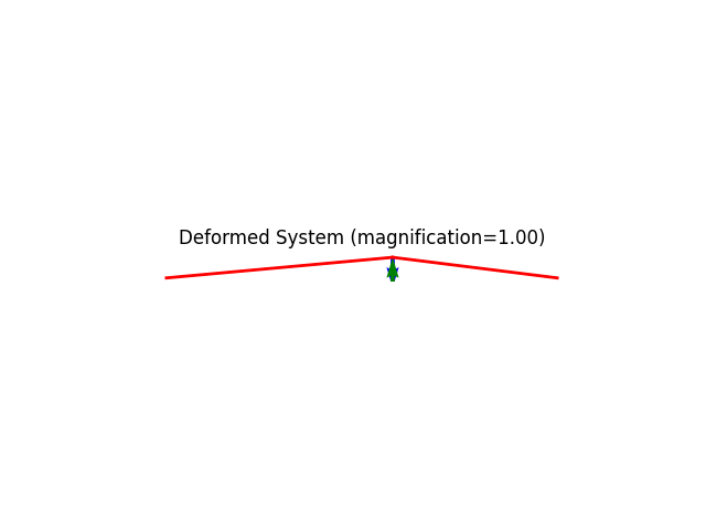
        model.plot(factor=1., filename="truss05_deformed.png")

        #
        # performing the analysis
        #
        model.resetDisp()

        # setting target displaement levels
        disps = np.linspace(0.0, 1.1, 24)

        # set up data collection
        load_list = []   # will hold load factors
        data_list = []   # will hold displacements

        # reset the analysis
        model.resetDisp()
        model.setLoadFactor(0.0)

        # apply all load steps
        for u_bar in disps:

            #model.setLoadFactor(lam)
            model.setDisplacementControl(x2, 'uy', -u_bar)
            model.solve()

            # collect data
            load_list.append(model.loadfactor)
            data_list.append(x2.getDisp())

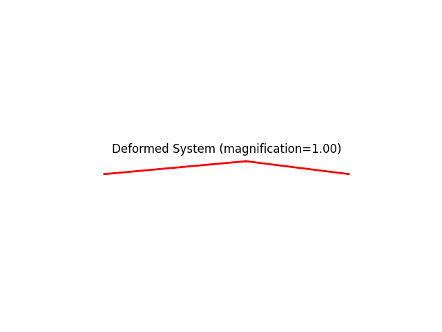
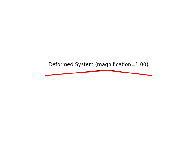
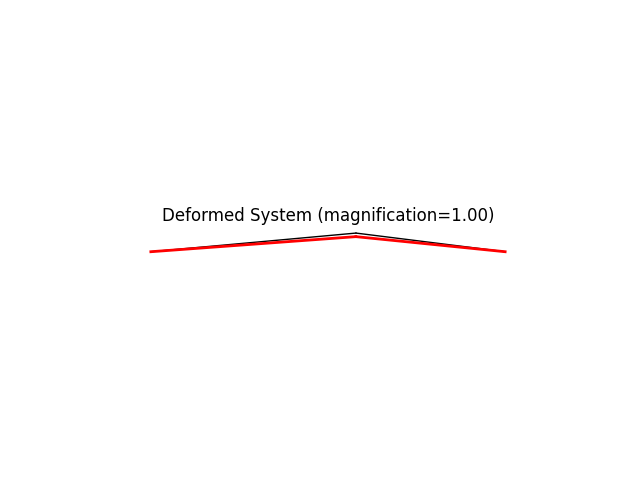
            # plot the deformed shape
            model.plot(factor=1.0, show_loads=False, show_reactions=False)

        load = np.array(load_list)
        data = np.array(data_list)

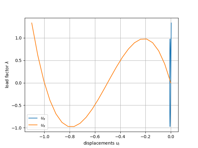
        plt.figure()
        plt.plot(data, load)
        plt.grid(True)
        plt.xlabel('displacements $ u_i $')
        plt.ylabel('load factor $ \lambda $')
        plt.legend(['$ u_x $','$ u_x $'])
        plt.show()

        #plt.figure()
        fig, (ax0,ax1) = plt.subplots(1,2)

        ax0.plot(load, data[:,0])
        ax0.grid(True)
        ax0.set_xlabel('load factor $ \lambda $')
        ax0.set_ylabel('displacements $ u_i $')
        ax0.legend(['$ u_x $'])

        ax1.plot(load, data[:,1])
        ax1.grid(True)
        ax1.set_xlabel('load factor $ \lambda $')
        ax1.set_ylabel('displacements $ u_i $')
        ax1.legend(['$ u_y $'])

        plt.show()

Run the example by creating an instance of the problem and executing it by calling Example.run()

if __name__ == "__main__":
    ex = ExampleTruss06()
    ex.run()

• 
• 
• 
• 
• 
• 
• 
• 
• 
• 
• 
• 
• 
• 
• 
• 
• 
• 
• 
• 
• 
• 
• 
• 
• 
• 
• 

System Analysis Report
=======================

Nodes:
---------------------
  Node_48:
      x:    [0. 0.]
      fix:  ['ux', 'uy']
      u:    None
  Node_49:
      x:    [5.5 0.5]
      P:    [ 0. -1.]
      u:    None
  Node_50:
      x:    [9.5 0. ]
      fix:  ['ux', 'uy']
      u:    None

Elements:
---------------------
  Truss: Node_48 to Node_49:
      material properties: FiberMaterial(Material)({'E': 2100.0, 'A': 1.0, 'nu': 0.0, 'fy': 1e+30})  strain:0.0   stress:{'xx': 0.0, 'yy': 0.0, 'zz': 0.0, 'xy': 0.0}
      internal force: 0.0
  Truss: Node_50 to Node_49:
      material properties: FiberMaterial(Material)({'E': 2100.0, 'A': 1.0, 'nu': 0.0, 'fy': 1e+30})  strain:0.0   stress:{'xx': 0.0, 'yy': 0.0, 'zz': 0.0, 'xy': 0.0}
      internal force: 0.0

+
+
+
+
+
+
+
+
+
+
+
+
+
+
+
+
+
+
+
+
/Users/pmackenz/Development/Educational/FEM.edu/src/femedu/plotter/ElementPlotter.py:119: RuntimeWarning: More than 20 figures have been opened. Figures created through the pyplot interface (`matplotlib.pyplot.figure`) are retained until explicitly closed and may consume too much memory. (To control this warning, see the rcParam `figure.max_open_warning`). Consider using `matplotlib.pyplot.close()`.
  fig, axs = plt.subplots()
+
+
+
+