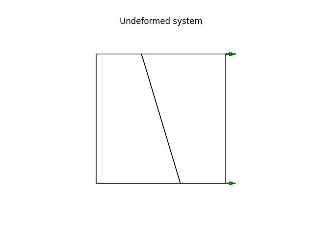
A square patch made of one quadrilateral plate elements

Basic implementation test with applied loads.

Testing the tangent stiffness computation.

free   free
 ^     ^
 |     |
 3-----2 -> free
 |     | >
 |  a  | > (w = 1.0)
 |     | >
 0-----1 -> free

width:  10.
height: 10.

Material parameters: St. Venant-Kirchhoff, plane stress
    E  = 10.0
    nu =  0.30
    t  =  1.0

Element loads:
    node 0: [ 0.0, 0.0]
    node 1: [ 5.0, 0.0]
    node 2: [ 5.0, 0.0]
    node 3: [ 0.0, 0.0]

Author: Peter Mackenzie-Helnwein

import numpy as np

from femedu.examples import Example

from femedu.domain import System, Node
from femedu.solver import NewtonRaphsonSolver
from femedu.elements.linear import Quad
from femedu.materials import PlaneStress


class ExamplePlate08(Example):

    # sphinx_gallery_thumbnail_number = 2
    def problem(self):

        params = dict(
            E  = 10., # Young's modulus
            nu = 0.3,   # Poisson's ratio
            t  = 1.0,   # thickness of the plate
            fy = 1.e30  # yield stress
        )

        a = 10.     # length of the plate in the x-direction
        b = 10.     # length of the plate in the y-direction
        c = 1.5

        model = System()
        model.setSolver(NewtonRaphsonSolver())

        nd0 = Node( 0.0, 0.0)
        nd1 = Node(a/2+c,0.0)
        nd2 = Node(   a, 0.0)
        nd3 = Node( 0.0,   b)
        nd4 = Node( a/2-c, b)
        nd5 = Node(   a,   b)

        # nd0.fixDOF('ux', 'uy')
        # nd1.fixDOF('uy')
        # nd2.fixDOF('uy')
        # nd3.fixDOF('ux')

        model.addNode(nd0, nd1, nd2, nd3, nd4, nd5)

        elemA = Quad(nd0, nd1, nd4, nd3, PlaneStress(params))
        elemB = Quad(nd1, nd2, nd5, nd4, PlaneStress(params))

        model.addElement(elemA, elemB)

        #elemA.setSurfaceLoad(face=3, pn=1.0)
        elemB.setSurfaceLoad(face=1, pn=1.0)

        model.plot(factor=0.0, title="Undeformed system", filename="plate08_undeformed.png", show_bc=1)

        # %%
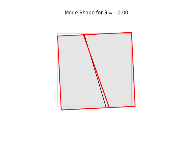
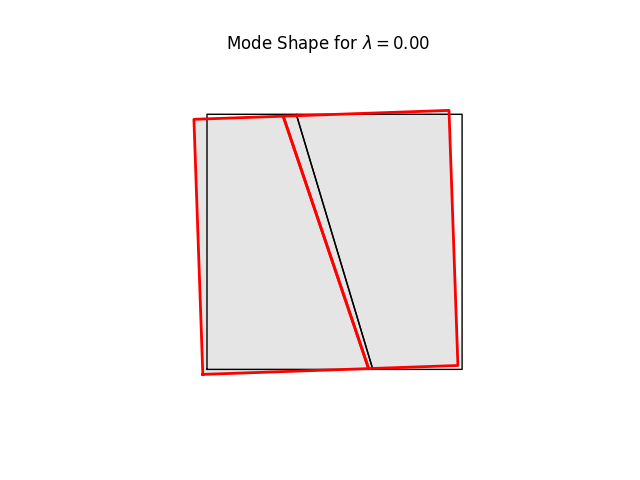
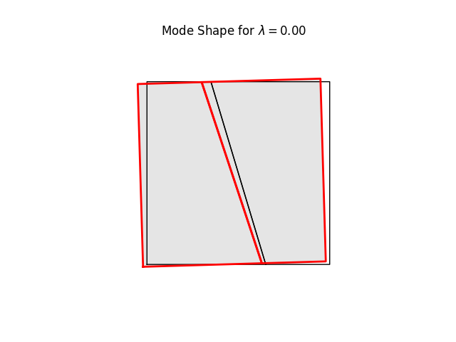
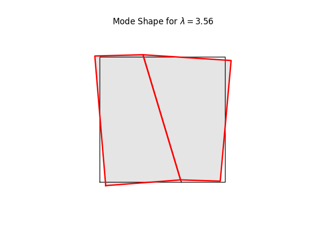
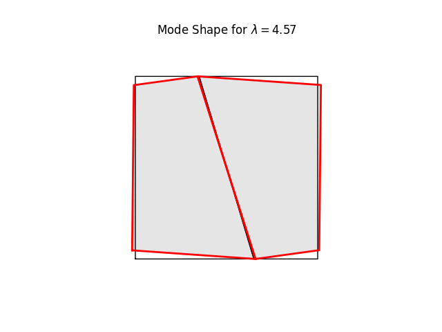
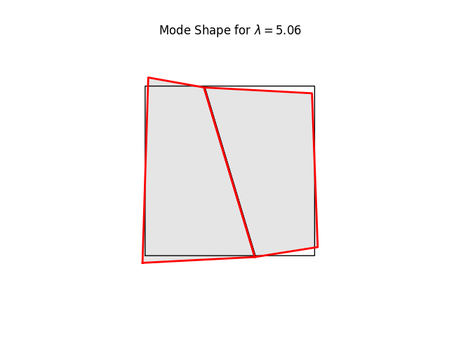
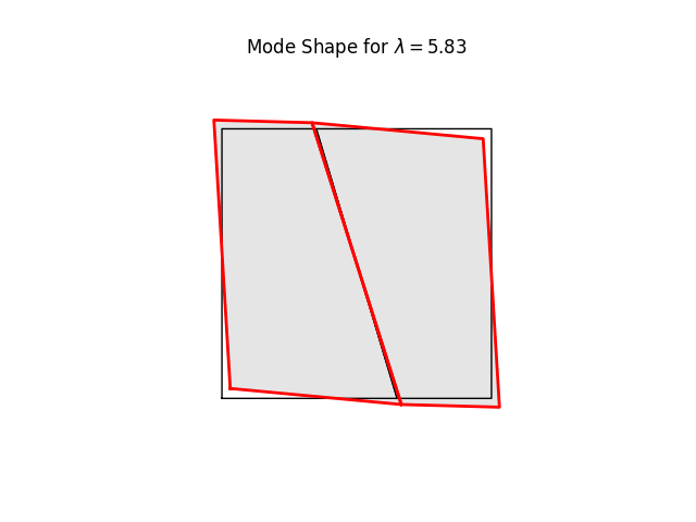
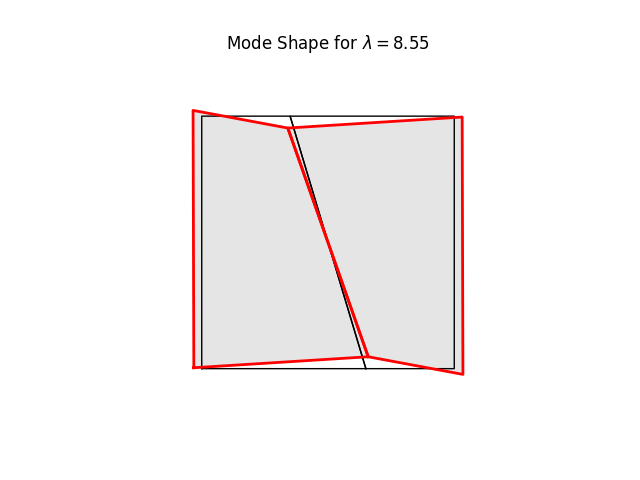
        # We can have a quick look at the stiffness mode shapes using the
        # buckling-mode plotter.  These are simply eigenvalues and eigenvectors of Kt
        # at the current load level (0.0)
        #
        model.setLoadFactor(0.0)
        model.solve(tol=1000.)

        for k in range(8):
            name = f"plate08_mode{k:2d}.png"
            model.plotBucklingMode(mode=k,filename=name,factor=1.0)

        # %%
        # Note the three rigid body modes (lam=0.0). It can be shown that all three
        # are limear combinations of translations in x and y-directions and a
        # rigid body rotation.
        #

        # %%
        # Now it is time to add boundary conditions, apply loads
        # and check the convergence behavior.
        #

        nd0.fixDOF('ux', 'uy')
        nd1.fixDOF('uy')
        nd2.fixDOF('uy')
        nd3.fixDOF('ux')

        model.setLoadFactor(1.0)
        model.solve()

        # %%
        # The output shows that we do have a quadratic rate of convergence.

        # %%
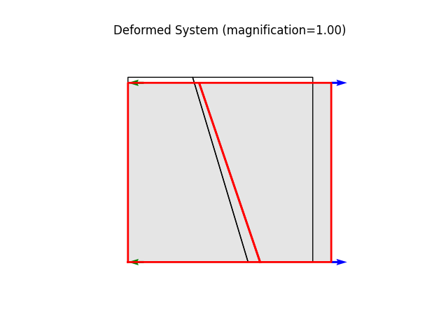
        # Let's finish off with a nice plot of the deformed system.

        model.plot(factor=1.0, filename="plate08_deformed.png")

        #model.report()

Run the example by creating an instance of the problem and executing it by calling Example.run()

if __name__ == "__main__":
    ex = ExamplePlate08()
    ex.run()

• 
• 
• 
• 
• 
• 
• 
• 
• 
• 

+
+